Unit conventions in the FHNC-app

I often have to do unit conversions, to compare to other work or to experiments. When doing this, I always have the feeling it takes more time than it should, because I have done these conversions already several times and they are simple. To make this process faster and easier for the users of the FHNC-app and for me, I state the conventions here.

Lets start with a simple example, the distance \(r\). This symbol represents a physical quantity, i.e. a number which multiplies a unit. Solving a physical problem on a computer we only use numbers, the information about the units has to be kept somewhere else. To make manipulations more transparent I split physical quantities: \(r=\tilde{r}r_s a_B\), where \(\tilde{r}\) is the variable implemented in the computer program and \(r_s a_B\) is the unit, the “typical” distance between two particles. The Hamiltonian of the HEG is then given by

$$H = \left(\frac{\partial^2}{r_s^2 \partial \tilde{\bf{r}}^2} + \frac{2}{r_s }\sum_{i<j}\frac{1}{|\tilde{\bf{r}}_i-\tilde{\bf{r}}_j|}\right)Ry$$

where Ry is the Rydberg energy. For other types of interaction the same units are used, although this is a bit unconventional. Often used units are then the Fermi energy and momentum, \(E_F\) and \(k_F\) respectively. The conversion is done with the dimensionless factor \(\alpha_d\), where \(d\) stands for the dimension. For 3D systems we have \(\alpha_3=\left( \frac{4}{9\pi} \right)^{\frac{1}{3}}\). With this we obtain

$$E_F=\frac{1}{\alpha_d^2 r_s^2}Ry \quad \text{and }\quad k_F= \frac{1}{\alpha_d r_s a_B} $$

Having a different mass of the particles \(m^*\), compared to the electron mass \(m\) is also covered, simply replace the units by starred ones:

$$ Ry^*= \frac{m^*}{m}Ry \quad \text{and }\quad a^*_B= \frac{m}{m^*}a_B$$

In dealing with this units stuff the book of Giuliani and Vignale: “Quantum theory of the electron liquid” is always a helpful resource.

The interactive FHNC-app is online!

I’m working a lot with plotly dashboards in the last months and I thought it would be nice to create an interactive FHNC-app with this technology. The result can be found here: https://fhnc-app.herokuapp.com/

The app calculates the static structure function (and pair distribution function) on the fly with the FHNC method. (one Boson and two Fermion approximations are implemented) Currently only the Coulomb interaction in 3D is implemented. Depending on the density parameter the calculation takes some seconds, higher rs-values take usually longer.

I’m planing to add other types of interaction and temperature dependence. If you have interest in a particular problem simply contact me by email or leave a comment here.

Recent Talks at 20th RPMBT and 24th ETSF-Workshop

In September I had the opportunity to give a talk at two influential and renown conferences, the 20th Recent Progress in Many Body Theories in Toulouse (France) and the 24th ETSF-Workshop in Jena (Germany). I presented an idea of how to systematically improve KS-DFT. The slides of the talk can be found here: talk

Results for Helium-3

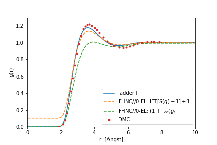
Recently I have feed our method1 (ladder+) with the Lennard-Jones potential. The parameters where chosen to resemble the Potential of Helium. (\(e=10.22K\) and \(\sigma=2.556\) Anst.) The result is excellent, as can be seen in the figure below:

The pair distribution function of He-3 in different approximations. The red dots are the DMC results of Casulleras and Boronat.2 The blue solid line is the ladder+ approximation. The dashed lines are two versions of the FHNC//0-EL given in Egger et al. 3

We compare to FHNC//0-EL, where the pair distribution is given by \(g(r)=(1+\Gamma_{dd}(r))g_F(r)\). Alternatively one could calculate the pair distribution from the Fourier-transform of the Static structure: \(g(r)=FT^{-1}[S(q)-1]+1\).

  1. 1.
    Panholzer M, Hobbiger R, Böhm H. Optimized correlations inspired by perturbation theory. Phys Rev B. 2019;99(19). doi:10.1103/physrevb.99.195156
  2. 2.
    Casulleras J, Boronat J. Progress in Monte Carlo Calculations of Fermi Systems: Normal LiquidH3e. Phys Rev Lett. 2000;84(14):3121-3124. doi:10.1103/physrevlett.84.3121
  3. 3.
    Egger J, Krotscheck E, Zillich RE. Bose and Fermi Gases with Lennard–Jones Interactions. J Low Temp Phys. 2011;165(5-6):275-291. doi:10.1007/s10909-011-0402-9

Article online

Our article “Optimized correlations inspired by perturbation theory” is now published: https://doi.org/10.1103/PhysRevB.99.19515

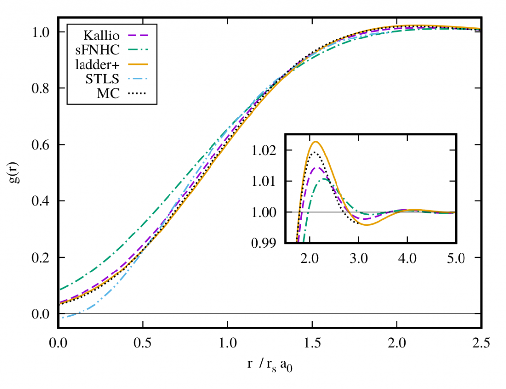
In the article we derive a simple approximation of the pair distribution function, which performs particularly well for the strongly correlated electron gas. It is the self-consistent solution of two equations:

\(\bigg[-\frac{\hbar^2}{m}\nabla^2 + v(r) + w_{\scriptscriptstyle\mathrm I}(r) +
V_{\scriptscriptstyle\mathrm F}(r)\, \bigg]_{\phantom{\big|}} \sqrt{g(r)} =\, 0 \) *

and

\(\tilde{w}_{\mathrm I}(q)=\, -\frac{\hbar^2 q^2}{4m} \left[\frac{1}{S(q)}-\frac{1}{S_{\mathrm{F}}(q)}\right]^2\left[\frac{2S(q)}{S_{\mathrm{F}}(q)}+1\right]\)

These two equations have a nice physical interpretation, the first eq. approximates the ladder diagrams and the second the ring (or bubble) diagrams. The result for the pair distribution function is shown in the figure below, for more details have a look into the article.

The pair distribution function at \(r_s=5\) in different approximations.

we used the relation \(g(r)-1 = \int \frac{d^3q}{(2\pi)^3\rho} e^{i{\bf q\cdot r}}\, \big(S(q)- 1\big)\).


  1. *
    with \(V_{\scriptscriptstyle\mathrm F}\equiv\frac{\hbar^2\nabla^2\sqrt{g_{\scriptscriptstyle\mathrm F}}}{m\sqrt{g_{\scriptscriptstyle\mathrm F}}}\)